
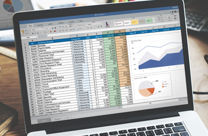
Want to add numbers quickly and easily in Excel? It turns out that there are three different ways of doing so. Watch this one-minute YouTube short video to find out.
Computer Training and Support

It turns out that there are three different easy ways to add numbers in Excel.
Want to add numbers quickly and easily in Excel? It turns out that there are three different ways of doing so. Watch this one-minute YouTube short video to find out.
In this video, we use the amazingly powerful VLOOKUP function to make it easier to keep track of the calories we consume.

Well, it took a while, but I finally finished the fourth and final part of my video series on Dieting with Excel. In this video, we use the amazingly powerful VLOOKUP function to make it easier to keep track of the calories we consume.
And as always, If you want to see the other videos in this series as well as several other videos and resources by Rich Malloy and Tech Help Today, be sure to click that same link: https://techhelptoday.com/videos/
To follow along, click https://techhelptoday.com/videos/ and click the link for the Excel workbook designed for this video.
Here’s a summary of the various parts in the Dieting Series:
Part 1: Dieting with a simple table
Part 2: Dieting with Excel Tables
Part 3: Dieting with Pivot Tables
Part 4: Dieting with the VLOOKUP function
 Microsoft has equipped the latest versions of Excel with some amazing “Power” features. In this hands-on Advanced Excel 2016 course taught by Rich Malloy at Norwalk Community College, students will learn how to use the most important of these industrial-strength tools: specifically, Power Query (also known as Get & Transform), Power Pivot, and Power View.
The course includes a review of Excel’s database features such as pivot tables, the VLOOKUP function, and the INDEX/MATCH combination. Students will also learn how to use Excel’s new formatted tables and slicers and how to take advantage of macros and the Visual Basic for Applications programming language.
![]() The six-session course will be held on Wednesday evenings from 6 pm to 9 pm. The first session is scheduled to start on April 10. Tuition is just $349. Go to www.norwalk.edu to sign up (use CRN number 5210), or visit the campus (directions).
The six-session course will be held on Wednesday evenings from 6 pm to 9 pm. The first session is scheduled to start on April 10. Tuition is just $349. Go to www.norwalk.edu to sign up (use CRN number 5210), or visit the campus (directions).
Microsoft has equipped the latest versions of Excel with some amazing “Power” features. In this hands-on Advanced Excel 2016 course taught by Rich Malloy at Norwalk Community College, students will learn how to use the most important of these industrial-strength tools: specifically, Power Query (also known as Get & Transform), Power Pivot, and Power View.
The course includes a review of Excel’s database features such as pivot tables, the VLOOKUP function, and the INDEX/MATCH combination. Students will also learn how to use Excel’s new formatted tables and slicers and how to take advantage of macros and the Visual Basic for Applications programming language.
![]() The four-session course will be held on Wednesday evenings from 6 pm to 9 pm. The first session is scheduled to start on Monday, October 29. Tuition is just $249. Go to www.norwalk.edu to sign up (use CRN number 6809), or visit the campus (directions).
The four-session course will be held on Wednesday evenings from 6 pm to 9 pm. The first session is scheduled to start on Monday, October 29. Tuition is just $249. Go to www.norwalk.edu to sign up (use CRN number 6809), or visit the campus (directions).
 The Charts & Graphs feature of Microsoft Excel is one of the app’s most popular features. With a few mouse clicks, you can create an decent chart. With a few more, you can create a really impressive one.
To help you create charts, we have put together a handy one-page Tips Sheet and an exercise file showing the three most popular types of charts.
The Advanced Budget Project — Part D: The Budget Report
A budget is probably the most important spreadsheet you can create. A good budget will keep you focused on your ultimate financial goal and help you avoid pitfalls like that adorable timeshare on Aruba.
 Now we are at the last part of our four-part Advanced Budget Project for Microsoft Excel 2016 on Windows. This is the crucial part where we find out how we are doing relative to our budget. In the first three parts, we created the Budget itself, a Ledger to keep track of our expenditures, and a Pivot Table to summarize our actual expenditures.
In this part, we will set up the all-important Budget Report, that is, a comparison of budgeted versus actual expenses. After going through the trouble of recording all of our expenses, this Budget Report will tell us if we are on budget or not. The pivot table we created in the last part already gives us a good summary of our expenditures. Ideally, we would like to insert some columns into the pivot table where we could display the budget estimates right next the actual expenses. Unfortunately, pivot tables are too inflexible for this. We could copy the pivot table values into a second table that would be more flexible, but this starts getting complicated real fast. Fortunately, there is much more direct way.
If we want to compare our actual expenditures with our budget, we need to summarize our actual amounts, and the best way to do that is with an Excel function called SUMIFS. You may already be familiar with the SUMIF function, which is handy for adding up numbers that meet a certain condition. And yes, if all we wanted was to find the total expenses in each category and did not care about the month, the simple SUMIF function would be fine.
But for our summary, we want to add up the expenses based on two conditions, Category and Month. For example, we want to see the total Groceries expenses for each individual month: Jan, Feb, and Mar. The SUMIFS function is perfect for this. Unlike the simple SUMIF function, it can add up items according to any number of different conditions. And unlike the pivot table, the SUMIFS function updates itself automatically. Think of that last “S” in SUMIFS as standing for “Super”.
Because of space considerations, we will do a Budget Report only for the first quarter of the year. The procedures for the other quarters are exactly the same.
As mentioned above, this project was done using Excel 2016 (updated by Office 365) running on Windows 10. Most if not all aspects of this project can be performed on other versions of Excel, but the exact instructions may differ.
In the first two parts of our Advanced Budget Project for Excel 2016 in Windows, we set up the Budget itself and then created a Ledger table to keep track of our expenditures. In the Ledger table, we set up filters using Excel’s Slicers so that we could see the total expenditures for each expense category and each month. The Slicer buttons are slick, but it will be tedious to use them to examine every single category and every month. There must be a better way.
And there is, of course. The fastest and easiest way to summarize a table is to use Excel’s PivotTables. This amazing feature has somehow obtained the reputation of being difficult, but I will let you in on a secret: Even though Pivot Tables are incredibly powerful, they are also surprisingly easy.
In this third part of our Advanced Budget project, we will set up a Pivot Table to see how the expenditures in our Expense Ledger are doing. In just a handful of mouse clicks, we’ll be able to peruse a summary of total expenses for all categories and months at the same time. We’ll also use two Excel features to give us a visual summary of our expenditures. Sparklines will show us a basic look at how our expenditures vary month to month, while a Pivot Chart will give us a much more detailed look.
Once you create a Pivot Table, you will be amazed at how easy it was. But don’t tell anyone. Let everyone continue to believe that this feature is too difficult for most people. And, of course, they will all be very impressed when you create them so quickly.
For instructions on Creating a PivotTable, click here.
For complete instructions on the Advanced Budget Project along with other projects in our Advanced Excel Course, click here.
— Rich Malloy
Having a budget is a great first step. Now that we created a budget in the first part of this project, we must follow that budget, or at least try to. This means categorizing and adding up perhaps hundreds of expenses throughout the year. As we shall see, Excel has special functions that will make categorizing and adding a breeze. But first we have to record all the expense data into a table we call the Ledger.
A Ledger is simply a record of all income and expenses. In this part of the project, we will create a ledger for expenses. Later the fun will begin when we conjure up some special magic in Excel to see if we are on — or off — budget.
For instructions on Creating a Ledger, click here.
For complete instructions on the Advanced Budget Project along with other projects in our Advanced Excel Course, click here.
A budget is probably the most important spreadsheet you can create. A good budget will keep you focused on your ultimate financial goal and help you avoid pitfalls like that adorable timeshare on Aruba. Budgets are surprisingly popular among rich people. You would think that wealthy people have so much money that they do not need a budget. But according to the book The Millionaire Next Door by Thomas J. Stanley and William D. Danko, most wealthy people in fact do have budgets, which may be part of the reason why they are rich in the first place.
In this project, we are going to set up not only a budget, but also a ledger to keep track of expenses and a budget report to show how our actual expenditures compared with our budget. This project presents an ideal case for taking advantage of some of the more advanced features of Excel.
In this first part of our Advanced Budget Project, we are going to set up the actual budget. A budget is simply a plan, in this case a plan for getting and spending money. Like all plans, budgets do not fare extremely well when they come up against reality. But that may not entirely be the point. President and five-star general Dwight D. Eisenhower once said, “In preparing for battle I have always found that plans are useless, but planning is indispensable.”
The Mail Merge feature of Microsoft Word is a great way to produce a large number of personalized letters or labels in a short amount of time. The process can seem daunting to a beginner, but if you break it down into a series of steps, is very easy to manage.
The Mail Merge feature of Microsoft Word is a great way to produce a large number of personalized letters or labels in a short amount of time. The process can seem daunting to a beginner, but if you break it down into a series of steps, is very easy to manage.
![]() The Mail Merge process basically involves taking two files and merging them together. The first file is a letter, which is a basic word document. The second is a list of recipients. This list could be a table in Microsoft Word, but most often it is a worksheet in Excel. In this example, we will use an Excel spreadsheet and a simple letter that has already been created in Word.
The Mail Merge process basically involves taking two files and merging them together. The first file is a letter, which is a basic word document. The second is a list of recipients. This list could be a table in Microsoft Word, but most often it is a worksheet in Excel. In this example, we will use an Excel spreadsheet and a simple letter that has already been created in Word.
The list of recipients is simply a table of names and addresses. There must be only one row of column headers at the top of the table, and each column headers should be unique. It will save some time later if you use a few standard labels in the column headers, such as, Last Name, Street, City, etc. I have prepared a very simple table of names and addresses in the file Mail_Merge_Recipients.xlsx. If you look carefully, you will note that the Postal Code column is set as text, which is why the ZIP codes appear on the left side of the cells. Unfortunately, this is mandatory: You must set the Postal Code column as text. Otherwise the leading zeros that are used in certain U.S. ZIP codes will be truncated off by Excel when it exports it to Microsoft Word. (This problem will occur even if you use the special Zip Code format of Excel.) Close the Excel file and proceed to the next step.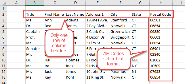
You can use almost any document in Mail Merge. I have prepared a simple letter with the file name Mail_Merge_Letter.docx. The date near the top is set to update every time we create a new batch of letters, which is a good idea for a Mail Merge letter. There is a placeholder for the Inside Address and another for the salutation line. (We could also put some information from the recipient list into the body of the letter. For example, we can add the line, “I hope things are going well in X,” Where X would be substituted by the recipient’s city. But such simple-minded gimmicks impress nobody, and for this example we’ll keep things simple.)
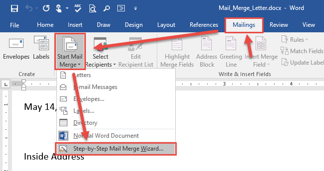
In Microsoft Word, if you want to start a Mail Merge, you will of course go to the Mailings tab. In that tab, click the button: Start Mail Merge. A menu of possibilities appears, and easiest choice is to go to the bottom and employ the Step-by-Step Mail Merge Wizard. So far, pretty simple, right?
 4. Choose the Document Type
The Mail Merge Wizard has just six steps, the first of which is the easiest. It defaults to creating a letter, which is exactly what we want. So, all you need to do is go to the next step. Click the button at the bottom right-hand corner: Next: Starting document.
We already have our document open, so all we need to do is click Next: Select recipients. (I told you it was easy!)
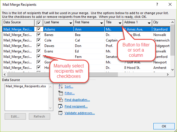
Now we choose the second ingredient in our Mail Merge recipe, the list of recipients. Click the Browse button and browse to the Excel spreadsheet that we looked at earlier. A dialog box should open up, showing all of the rows and columns of our Excel spreadsheet. To the left of each row there are checkboxes which we can use to manually select who should receive our letter. Also, note that each of the column headers has a filter button, a drop-down arrow which we could use to select which groups of recipients will receive the letter. (We could also use these filter buttons to sort our letters. In some cases, we can get discounted postal rates if we were to sort the letters in the order of their ZIP Codes.) In this example will leave all our recipient selected so that everyone will receive one of our amazing letters. Click OK to close the dialog box, and then click Next: Write your letter.
 7. Write the Letter
Well, our letter is pretty much already written. But we do need to add two things: the inside address, and the salutation or greeting line. Delete the text that says Inside Address and leave the mouse pointer on that line. In the Mail Merge task pane at the right, click the option: Address block. A dialog box will appear asking you to confirm that the name and address information is correct. After you click OK, a merge field code will appear in your letter. This code is distinguished by the double angle brackets that enclose it. As with all fields, Microsoft Word will replace it with some relevant information, in this case, a few lines that list the name and address of the recipient. Because we used standard labels in the column headers of our Excel spreadsheet, Word knows how to combine the name and address information in a suitable way. (If we had not used standard labels, we would now have to tell Word which of our labels corresponds to the standard labels, so that Word could assemble the address block as needed.)
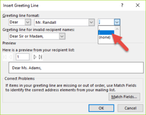 Next, we have to add the salutation or greeting line. Delete the text now in the salutation and click the Greeting line option in the task pane on the right. A dialog box will appear asking you to confirm the structure of the salutation. Because this is a business letter, we need to change the punctuation to a colon. Click the list arrow at the right near the comma and change it to a colon. Then click OK.
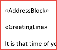 In this step, we have added two merge fields. Be sure there is a blank line below each merge field. It looks a little cryptic right now, but that will soon change—as soon as you click Next: Preview your letters.
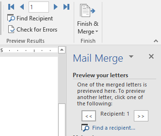 Prepare to be amazed: In this step, the merge fields have been replaced with actual data. You can use the arrow buttons to move forward or backward in your recipient list to see how each of the letters will appear. If you see any mistakes regarding line spacing or word spacing in the salutation, this is a good chance to fix that. Assuming that everything looks fine, let’s go on to the next step. Click Next: Complete the merge.
Before we do the actual merge, it’s a good idea to save our work: Press Ctrl + S. Now, as you can see in the task pane on the right, there are two basic choices. If everything looks pretty good so far, you can take a chance and click the button: Print. This will merge our letter with our recipient list and print out X number of letters. But if there’s a mistake someplace in the letter, you may print out X number of mistakes.
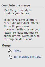 If you’re the more cautious type like me, the better choice is: Edit individual letters. This creates a new document which is composed of all the individual letters that are created in the Mail Merge process. We can now go through this batch of letters and correct any mistakes. We could also add a little personalization to a particular letter, for example, “I enjoyed seeing you at the park last week.” After we make our choice, Word will ask you to confirm that you want to print all the letters, which you usually want to do.
In the new “Letters” document that appears, note that each of the letters is separated not by a Page Break, but by a Section Break (Next Page). This means that each of the individual letters are actually sections of the document. I’m not sure why Microsoft chose to break up the letters this way, but it does have an important consequence for us: If we want to print only certain letters in the document, we would specify not their page numbers, as we would usually do. Instead, we must specify the section numbers. That is, instead of entering 1, 4, 7, in the box for Pages to be printed, we would instead enter: S1, S4, S7.
Let’s assume that all the letters look fine, and we have plenty of paper and ink in our printer. What we need to do now is print the Letters document. Once it is printed, the Letters document is no longer needed. We can use the original letter document we just saved a moment ago to create a new collection of letters in just a few mouse clicks. So, close the Letters document without saving it. The original mail-merge letter document will now appear, and that should be saved for possible reuse in the future.
Well, it turned out to be even easier than I thought. Really only nine steps! Practice this a few times, and pretty soon you’ll be able to do it all by yourself—without the wizard.
Of course, there is one more step: If we want to mail these letters, we need to print either labels or envelopes. Sorry, we’ll have to leave that for another lesson.
— Rich Malloy